A lot of time I’ve come across the weak form of PDEs for physical systems, particularly for physics simulations. And just searching for “weak formulation of PDEs” led me into deep rabbit holes where I’d quickly feel lost and overwhelmed.

Then I saw notes “A brief introduction to weak formulations of PDEs and the finite element method” by Prof. T. J. Sullivan. He really nicely put the why behind all of the weak formulation. Primary concepts I learned are:

• The strong form is often too rigid for PDEs for physical simulation, which are either not tractable or don’t even have solutions for given constraints. So weak form is a less rigid version of such PDEs where the smoothness and continuity requirements are often relaxed by paring them against some test function.
• This weak formulation by test function + integration by parts lets us formulate 2nd order elliptical PDE (Poisson equation) into 1st order.
• One interesting thing I noticed, the space of all test functions forms a vector space, which is perfect candidate for writing the weak formulation in exterior calculus notation.

Strong Formulation

To begin with, let’s consider a 2^nd order elliptical PDE, the Poisson problem over a subset of euclidean space such that $\mathcal{D} \subset \mathbb{R}^n$. Where $u: \mathcal{D} \to \mathbb{R}$, $f: \mathcal{D} \to \mathbb{R}$ are function over the domain. Then a strong form of Poisson equation is

$$\begin{matrix} \Delta u(x) = f(x), \quad \forall x \in \mathcal{D} \\ f(x) = 0, \quad \forall x \in \partial\mathcal{D} \end{matrix}$$

Weak Formulation

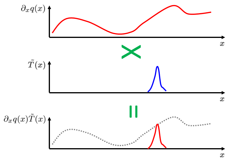
Let $\phi: \mathcal{D} \to \mathbb{R}$ be a compactly supported test function. This is cumbersome, but what it means is that $\phi$ is infinitely differentiable and is non-zero only over some subset of $\mathcal{D}$. More precisely, There exists some closed and bounded set $S \subset \mathcal{D}$ such that $\phi$ is zero over $\mathcal{D} \setminus S$. Why this matters? #look-into-it.

Now let’s pair $\phi(x)$ with our strong form, then the weak form becomes:

$$\int \Delta u(x) \phi(x) dx = \int f(x) \phi(x) dx \quad \forall \phi \in \mathcal{C}^{\infty}(\mathcal{D})$$

Then in a weak sense we are saying that $\Delta u(x) = f(x)$. If we pair this weak formulation with integration by parts, then we can relax the differentiability constraint on $u$.

With the integration by parts, we can rearrange the equation as,

$$\begin{equation} \int \nabla u(x)\nabla \phi(x)dx = \int f(x)\phi(x)dx \quad \forall \phi \in \mathcal{C}^\infty(\mathcal{D}) \tag{1} \end{equation}$$

This effectively makes out $u$ to be only $\mathcal{C}^1(\mathcal{D})$ rather than $\mathcal{C}^2(\mathcal{D})$. And I think this means that we can work with linear piecewise constant $u(x)$ and $\phi(x)$, for which we already have lot of numerical machinery from linear algebra in place.

Linear algebra connection

We can express Eq. $(1)$ using a bilinear Form and inner product

$$B(u, \phi) = \langle f, \phi \rangle_{L^2}$$

where $B$ is a linear function of $u$ and $\phi$ and $\langle f, \phi \rangle_{L^2}$ is a $L^2$ inner product given by

$$\begin{matrix} B(u, \phi) = \int \nabla u(x) \nabla \phi(x)dx \\ \\ \langle f, \phi \rangle_{L^2} = \int f(x)\phi(x)dx \end{matrix}$$

here we can see that $\langle f, \cdot \rangle_{L^2}$ is a covector and and $B(u, \cdot)$ is a differential form.

Sobolev Spaces

It’s a space of all scalar valued functions which are square integrable and their gradients are square integrable as well. (i.e. $\int_{D}\lvert u(x) \rvert^2dx$ is finite). Why this matters? #look-into-it

This space is denoted by $H^1(\mathcal{D})$ an is equipped with an inner product structure

$$\langle u_{1}, u_{2} \rangle_{H^1} = \int_{\mathcal{D}}u_{1}(x)u_{2}(x)dx + \int_{\mathcal{D}}\nabla u_{1}(x)\nabla u_{2}(x) dx$$

and a norm

$$\lVert u \rVert^2_{H^1} = \int_{\mathcal{D}}\lvert u(x) \rvert^2dx + \int_{\mathcal{D}}\lvert \nabla u(x) \rvert^2 dx$$

It seems like $L^2(\mathcal{D}) \subset H^1(\mathcal{D}))$. #look-into-it

Galerklin’s method and finite elements