Regularized Point Vortex Dynamics

Why Regularize?

The original point vortex dynamics, the point vortices are represented as delta functions $\delta_{p}$ . Then, from the in-compressible Eulerian fluid flow, we have a Poisson problem setup as:

$$- \Delta \psi = \omega, \quad \omega = \sum_{i=1}^N \Gamma_{i} \delta_{p_{i}}$$

The solution for this PDE is given by a Greens function. But this greens function has logarithmic singularities at the point vortex location.

$$G(x, p_{i}) \sim \log\left( d(p_{i}, x) \right)$$

Where $d(p_{i}, x)$ is geodesic distance.

The one big issue with is that the energy $\frac{1}{2} \int_{M}\lvert \nabla u \rvert$, which is equivalent to $\frac{1}{2}\int_M\psi \omega$ on a surface. As $\psi$ has a log singularity at $p_{i}$, the energy is infinite as well. Which also means the Hamiltonian of the system is infinite as well.

Regularized Point Vortex

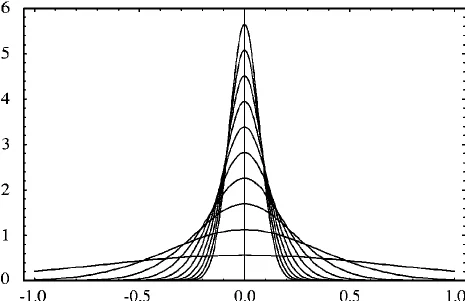
To solve this issue we define a point vortex as a blob with compact support $\epsilon$, now this limits the energy to be finite everywhere. And due to the radial symmetry of the blob, to points outside the core of the blob, the effect is same as of a point vortex to the leading order with error term of $O(\epsilon^2)$.

Let $M$ be a closed surface and let $G(x, y)$ be the Green’s function.

A vorticity for a point vortex at a point $a$ is defined as:

$$\omega = \Gamma_{i}\delta_{p_{i}}, \quad \psi = \int_{M} G(x, y) \omega dA_{x} = \Gamma_{i} G(p_{i}, y)$$

Now for a regularized point vortex blob:

$$\Gamma = \int_{M}\omega_{\epsilon}dA, \quad \psi=\int_{M}G(x, y)\omega_{\epsilon}(x)dA_{x}$$

Non Singular Stream Function

Averaging Green’s function over some area remove the singularity. The greens function has a logarithmic response for a point impulse, we can think of integrating such point impulses over an area. Zooming in around the singularity:

$$\psi = \int_{\epsilon} a\lvert \log r \rvert dA$$

Using polar coordinates around the point, $dA = r\, dr\, d\theta$. Then the integral becomes:

$$\psi_{\epsilon} = \int_{0}^{2\pi} \int_{\epsilon} a \lvert \log r \rvert r\,dr\,d\theta$$

and the $r \lvert \log r \rvert$ is finite over small path around origin, which explains why the average of singular greens function over a patch is not singular.

Difference in Point Vortex Vs Regularized Vortex Core

For getting a finite Hamiltonian we can regularize the Point vortex model to have a vorticity spread over a small neighborhood around the point, formally a compact support over a radially symmetrical code with radius $\epsilon$. Then the question becomes how does our fluid dynamics is affected by it. This can be quantified by comparing resultant stream functions $\psi$ in both cases.

For point vortex $\psi = \Gamma\, G(x, a)$ where there’s a point vortex at $y=a$. For a regularized point vortex we have, $\psi_{reg} = \int_{M}G(x, y)\,\omega_{\epsilon}(y)\,dA$.

Now for the regularized blob case we know that there’s no singularity present, i.e., green’s function is smooth near at the location of the point vortex core $a$. Using Taylor’s expansion we can write:

$$G(x, y) = G(x, a) + \nabla_{y}G(x, a) (y - a) + \frac{1}{2}(y-a)^T\Delta_{y}G(x, a)(y-a) + \dots$$

substituting this to get the regularized stream function,

$$\psi_{reg} = \Gamma G(x, a) + O(\epsilon^2)$$

As $\int(x-y)\,w_{\epsilon}(y)\,dA = 0$ for a radially symmetrical blob. But then,

$$\psi_{reg} = \psi + O(\epsilon^2)$$

Similarly, velocity is $u = \nabla_{x}\psi$, therefore:

$$u_{reg} = u + O(\epsilon^2)$$

Regularized point vortex dynamics is same to the leading order to the actual point vortex dynamics.

Regularization Due to Discretization

When we finally try to implement this continuum model on a discrete mesh we see a new form of regularization added by the coarseness of the mesh. Ideally the vorticity should be only supported on a ball of radius $\epsilon$ but once due to the splatting of the vortices to the mesh, we spread the actual vorticity on the basis vectors in the Finite Element space.

Spectral Decomposition of the Laplacian

TBD

• Taylor expansion of Green’s
  • Tells how blob is different from point
• Spectrum of Laplacian -> (eigen)modes of Laplacian -> Inverse using eigenmodes -> Explains smoothing -> adding heat kernel to filter -> Explains heat-kernel smoothing
• Implementation in the discrete case
• Simulation
  • Observe Hamiltonian
  • Observe error term wrt $\frac{h}{\epsilon}$.
• Complete the report and sent results to Albert!!!
• Regularization on continuum -> regularization due to mesh anisotropy -> fix -> implementation